Benchmark progress normalization
Fitting a logarithmic DeepSWE trend and a linear SWE-bench Pro trend gives 14.8 percentage points of time-equivalent Pro progress for the 79.0% → 82.3% DeepSWE gap.
The comparison asks: how much would the historical Pro trend advance over the interval that the fitted DeepSWE trend assigns to this gap?
This is a defined comparison of fitted historical progress. It is not a converted benchmark score, a relative percentage gain, or proof of equivalent task difficulty. Different time windows and curve assumptions change it; those checks are below.
Fit the record-setting results
All 63 Pro entries and 52 DeepSWE entries were retrieved. A new high on a model announcement date becomes one frontier record; duplicate entries and tied scores do not add fit weight. That yields six Pro records and eight DeepSWE records.
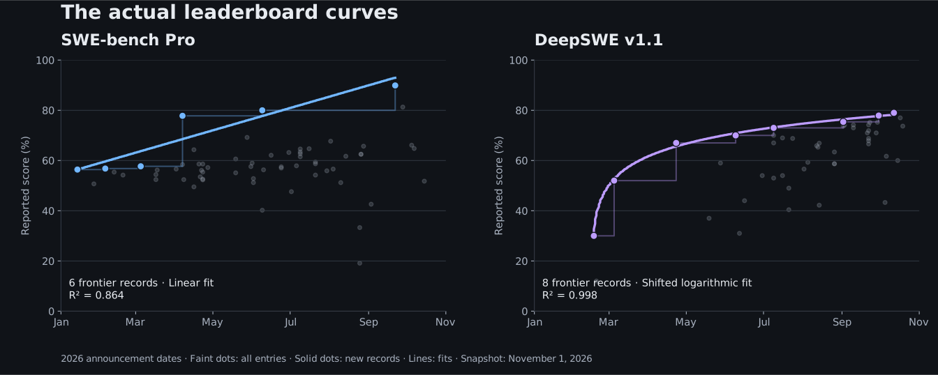
Descant’s published 82.3% result is the comparison target and is excluded from both fits. The 79.0% baseline is the highest listed DeepSWE result. Both pages label their listed results unverified; this calculation does not independently rerun the benchmarks.
The calculation
Scores are fractions and t is days since January 1, 2026. Ordinary least squares fits Pro to a line. DeepSWE uses a shifted logarithm; its time origin is fitted from the data, not chosen to produce 14 points.
The Pro intercept and starting date cancel in the difference. The DeepSWE time shift cancels explicitly in its inverse difference, while still affecting the fitted coefficients. This is the mathematical derivation of the number conditional on those two fitted curves.
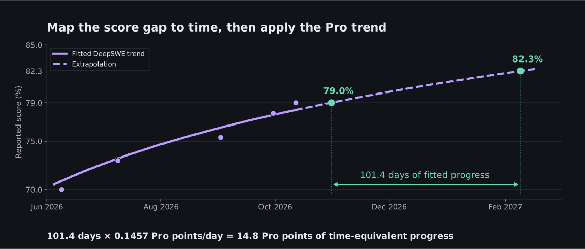
3.33 months of fitted DeepSWE progress × 4.44 Pro points per month = 14.8 Pro points
Exactly how the fit is obtained
For Pro, m = Σ(tᵢ − t̄)(pᵢ − p̄) / Σ(tᵢ − t̄)² and c = p̄ − m·t̄. For each candidate τ less than the earliest DeepSWE date, fit a and b by the same OLS formula with xᵢ = ln(tᵢ − τ), then minimize Σ[dᵢ − a − b·ln(tᵢ − τ)]² over τ. The script scans and refines a broad range of time offsets, 0.0001–36,500 days before the earliest point. The optimum is 1.881551 days before that point, well inside the bounds. Moving the calendar’s coordinate origin and τ together leaves the fitted curve unchanged.
Equal weight is assigned to each new record. Long plateaus are not copied into repeated daily observations. Fit R²: Pro 0.863968; DeepSWE 0.997614. Score residual RMSE: Pro 4.918 points; DeepSWE 0.764 points. R² describes the observed fit; it is not a probability that the extrapolation is correct.
How much does the method matter?
Anchoring the same curve to the latest observed 79.0% record gives 13.7 points. More substantial changes to the fitting window or curve produce a wider spread. This table is a sensitivity analysis, not a confidence interval.
| Calculation | Equivalent Pro points | What changes |
|---|---|---|
| Full-history shifted log + linear | 14.78 | Primary model; fit the time origin and invert both score levels. |
| Anchor DeepSWE curve to latest record | 13.67 | Same curvature, vertically shifted to pass through 79.0% on October 12. |
| Fix logarithmic origin at January 1 | 5.69 | An arbitrary fixed origin changes the fitted curvature; poorer fit (R² 0.898). |
| Omit earliest DeepSWE record | 16.66 | Seven records instead of eight. |
| Use April–October DeepSWE linear trend | 7.08 | Recent six DeepSWE records are also close to a line (R² 0.990). |
| Use April–September Pro linear trend | 7.53 | Only three Pro frontier records; its slope is lower than the full-history slope. |
Does the logarithmic curve have evidence beyond a high R²?
Fit only the earliest records, then predict the later records without refitting. The logarithmic curve describes this history much better than a full-history line. These small retrospective checks support the descriptive model; they do not validate its future extrapolation or establish a logarithmic benchmark scoring rule.
| Training → held-out records | Log RMSE (points) | Linear RMSE (points) |
|---|---|---|
| 4 → 4 | 0.66 | 28.51 |
| 5 → 3 | 0.74 | 20.81 |
| 6 → 2 | 1.04 | 10.80 |
| 7 → 1 | 1.05 | 6.55 |
Single-record deletion within the shifted-log family gives approximately 14.1–16.7 equivalent Pro points in an independent replication. Removing the first two records changes the shape much more: the April–October DeepSWE records are close to linear. The early rapid-improvement period matters to the 14.8 estimate.
What this does not establish
The logarithm models score progression over announcement dates; it does not mean DeepSWE is scored logarithmically. Its displayed score is a task-success proportion. Time-based progress is not a shared unit of capability, research effort, or engineering quality across benchmarks.
This is not a forecast of a Pro score above 100%. Adding 14.8 points to today’s 89.9% Pro leader would exceed that ceiling. The comparison uses a historical rate to express an interval, not an achievable future score.
The inputs combine model families, harnesses and configurations. Announcement dates can predate the publication of benchmark scores. Historical rows can be missing or revised. No task-level uncertainty or statistical-significance claim is inferred from the displayed aggregates.
A different question—fitting Pro score directly against DeepSWE score for shared model IDs—does not produce the same normalization. The shared models top out at 74.2% DeepSWE and have configuration differences. Neither that mapping nor this time-based one is a universal conversion between benchmarks.
Every fitted point
SWE-bench Pro
| Announcement | Model | Score |
|---|---|---|
| 2026-01-14 | GPT-5.2 Codex | 56.4% |
| 2026-02-05 | GPT-5.3 Codex | 56.8% |
| 2026-03-05 | GPT-5.4 | 57.7% |
| 2026-04-07 | Claude Mythos Preview | 77.8% |
| 2026-06-09 | Claude Fable 5 | 80.0% |
| 2026-09-22 | Claude Opus 5.5 | 89.9% |
DeepSWE v1.1
| Announcement | Model | Score |
|---|---|---|
| 2026-02-17 | Claude Sonnet 4.6 | 30.0% |
| 2026-03-05 | GPT-5.4 | 52.0% |
| 2026-04-23 | GPT-5.5 | 67.0% |
| 2026-06-09 | Claude Fable 5 | 70.0% |
| 2026-07-09 | GPT-5.6 Sol | 73.0% |
| 2026-09-02 | Muse Spark 1.3 | 75.4% |
| 2026-09-30 | Gemini 4 Argon | 77.9% |
| 2026-10-12 | Muse Wonder Full | 79.0% |
Reproduce it
Download the source snapshots and calculation, install the pinned dependencies, then run python analyze.py. It regenerates the coefficients, CSV records, sensitivity results and charts. No network calls are needed to reproduce the saved snapshot.
All 115 listed models are retained in the CSV inputs with their announcement dates, scores, verification status and source links. Unused provider metadata is omitted. Configuration details remain available from the linked sources; the original full payload is retained with the research archive. Results record hashes of these published CSV inputs. The separate independent calculation reproduced 14.7784 points using a different optimizer.